Electrical Tone and the Harmonic Idea
Section I · Theory
Build the modelSound, history, and the mathematics that connects them.Chapter contract
Prerequisites. Arithmetic with fractions, comfort reading simple graphs, and willingness to listen at a fixed safe level. No previous synthesis or trigonometry is assumed.
By the end of this chapter, you should be able to:
- find amplitude, frequency, phase, and period in a sine wave;
- calculate the frequencies in a harmonic series;
- explain the difference between a partial, harmonic, fundamental, and overtone;
- build and read a tone made from a finite number of sine waves;
- explain how harmonic balance affects a sustained tone while recognizing that timbre also changes over time;
- trace how the Helmholtz/Koenig apparatus and the Telharmonium generated, controlled, and reproduced sound;
- explain why the Telharmonium was similar to, but not identical to, modern additive synthesis;
- calculate cycle lengths, harmonic frequencies, finite sums, and which harmonics fit below the Nyquist limit;
- explain every numbered formula from its adjacent plot;
- render a short melody and a repeating timbre pattern with the browser lab.
The problem: why can one pitch have many colours?
Sing a steady vowel, then change the vowel without changing the note. Play the same written pitch on a flute and a bowed string. The perceived pitch can remain approximately stable while the identity and colour of the sound change dramatically.
That observation gives us the first design problem of synthesis:
If pitch does not uniquely determine sound, what else must an instrument control?
Nineteenth-century acoustics gave a testable answer. Many sustained musical tones can be modeled as simpler sine-wave components. When their frequencies follow a harmonic pattern, changing their relative amplitudes changes the tone colour. Helmholtz centered his account of tone quality on this relation. Rudolph Koenig built apparatus that made it audible (Helmholtz 1885; Rees 2010; “Helmholtz Synthesizer (Koenig)” n.d.).

Image credit and licence. Photograph by Jane023, 2012, showing an apparatus dated 1865 in the Teylers Museum instrument room. Creative Commons Attribution–ShareAlike 3.0 (Jane023 2012).
Long description. A museum case contains a horizontal row of electrically maintained tuning forks, each paired with a brass spherical resonator. Mechanical controls and a keyboard allow selected resonators to contribute to the combined sound. The apparatus makes an abstract synthesis equation physical: one path produces one component, a level or shutter controls whether it is heard, and the air adds all active components.
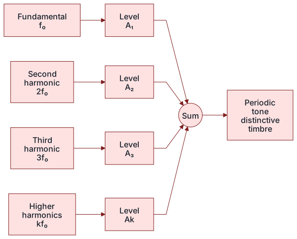
Its layout gives us a complete signal model:
component generator → component level → summing medium → compound toneOne basic building block: the sine wave
A sine wave is the simplest repeating waveform. It contains one frequency and no additional harmonic components. More complex repeating sounds can be described as sums of sine waves with different frequencies, amplitudes, and phases. Amplitude is the size of a wave, frequency is its number of cycles per second, and phase is its position within a cycle. The mathematical term for a sine wave is sinusoid (Smith 2011; Puckette 2007). We write one as:
| Symbol | Meaning | Unit |
|---|---|---|
| time | seconds | |
| peak amplitude | normalized linear amplitude | |
| frequency | hertz | |
| initial phase | radians |

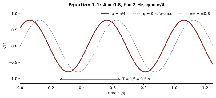
Long description. Time runs from 0 to 1.25 seconds. A solid sinusoid reaches peak amplitudes of ±0.8 and repeats every 0.5 seconds. A dashed zero-phase reference shows how shifts the cycle. A horizontal arrow marks one period.
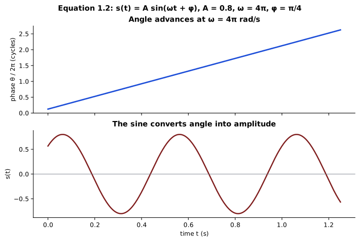
The value inside the sine function is an angle. A radian is a unit for measuring angle. One complete cycle contains radians. The term advances by that amount during every completed cycle. Phase chooses where in that cycle the signal starts. The same component can also be written with angular frequency :

Long description. The upper panel shows phase increasing linearly at two cycles per second. The lower panel applies sine to that angle and produces the same shifted 2 Hz waveform as Equation 1.1.
This is an ideal model: it deliberately leaves out the extra components and energy loss found in physical systems. Real tuning forks contain other components, resonators lose energy, and loudspeakers change the signal they reproduce. We start with a sine wave because it isolates one frequency and gives us a reference for more complicated tones (Smith 2011; Puckette 2007).
Period and frequency
Start with a 2 Hz sine wave. It completes two cycles in one second, so each cycle lasts half a second. The duration of one complete cycle is called the period, written .
More generally, frequency counts cycles per second. In seconds, the wave completes cycles. One period contains exactly one cycle, so .
The sine equation describes the same idea with angles. One cycle is radians. During seconds, the angle advances by radians. To complete one cycle, that advance must equal :
Ready. Play one cycle to connect one full turn with one period.
Long description. The top wave starts at zero. The lower wave starts later in its cycle, so its shape is shifted. Dashed lines mark two matching peaks on each wave. Both peak-to-peak intervals have length . A circle at the lower right connects one complete waveform cycle to one complete turn of radians.
Starting phase does not affect this result. It only chooses which point in the cycle appears at . Whether the wave starts at zero or at a peak, the time from one peak to the next is still .
Now remove the common factor by dividing both sides by it:
This says that the wave completes exactly one cycle during one period. To find the period, divide by . To find the frequency, divide it by :
In words: period is the number of seconds per cycle; frequency is the number of cycles per second. They are reciprocals. For example, a 2 Hz wave fits two cycles into one second, so each cycle lasts second.

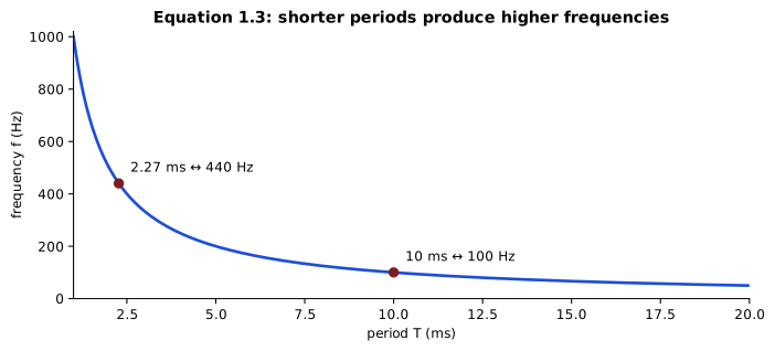
Long description. The reciprocal curve falls steeply at short periods and flattens at long periods. Markers identify the 100 Hz and 440 Hz examples. Moving right to a longer period always moves down to a lower frequency.
For a 100 Hz component,
For A4 at 440 Hz, one cycle lasts approximately
Sanity rule. Higher frequency means a shorter period. If your calculation gives a longer period for a higher frequency, the ratio has been inverted.
From one component to a harmonic family
A stable pitched tone often contains a fundamental frequency, written . This is the reference frequency that we hear as the basic pitch. A harmonic is a component whose frequency is a whole-number multiple of that fundamental (Wolfe n.d.; Puckette 2007):

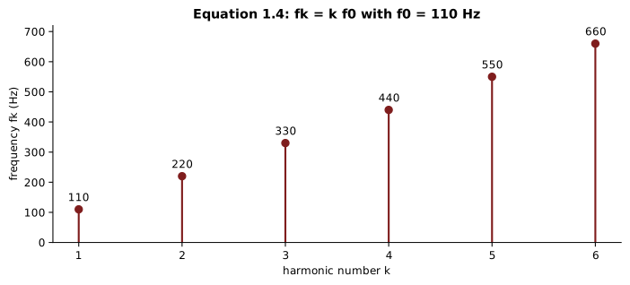
Long description. Six stems rise at harmonic numbers 1 through 6. Their labeled frequencies are 110, 220, 330, 440, 550, and 660 Hz. Equal horizontal steps in harmonic number produce equal 110 Hz vertical steps.
For Hz, the first six harmonic frequencies are:
110, 220, 330, 440, 550, 660 HzThese related words have different meanings (Wolfe n.d.; Helmholtz 1885):
- A partial is any frequency component of a tone.
- A harmonic partial lies at a whole-number multiple of .
- The fundamental is harmonic 1.
- An overtone is a component above the fundamental. The first overtone is therefore normally harmonic 2.
- Some physical instruments contain overtones that are not harmonic.
This distinction matters later. A wavetable frame is one stored waveform in a set of waveforms. In a strictly periodic oscillator, its frequency content lines up with harmonic positions, sometimes called harmonic bins. Bells, stiff strings, noisy attacks, and objects that resonate in several modes can also contain important inharmonic partials: components that do not fall at whole-number multiples of the fundamental.
Build a tone by adding sine waves
Additive synthesis builds one sound by adding controlled components. A finite model uses a limited number of them. For a repeating tone, we can write that model as a sum of sine waves (Smith 2011; Puckette 2007):
| Symbol | Meaning |
|---|---|
| number of modeled harmonics | |
| amplitude of harmonic | |
| frequency of harmonic | |
| phase of harmonic |
Every term completes an integer number of cycles during the fundamental period . Their sum therefore repeats after , unless a particular selection of terms implies an even shorter fundamental period.

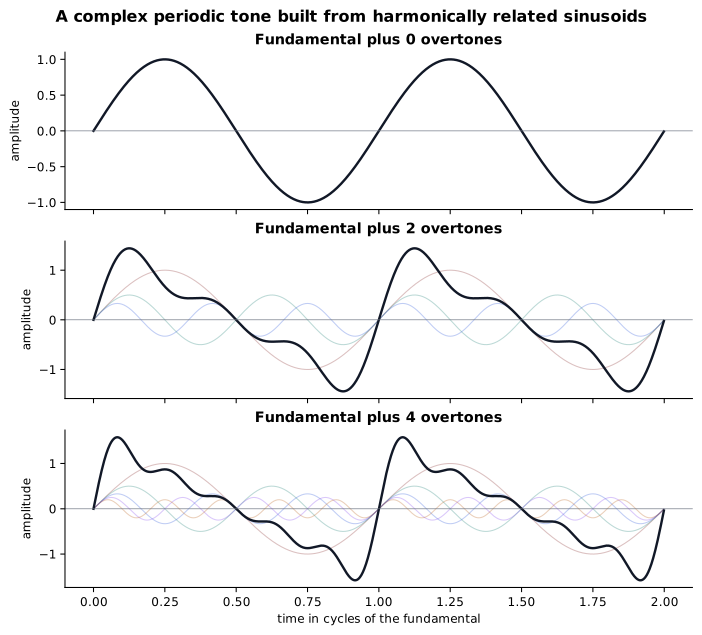
Figure provenance. Author-generated by
assets/figures/src/ch01_harmonics.py from Equation 1.5. The
plotted zero-phase amplitudes are
.
No measured or third-party data are used.
Long description. Three panels show two cycles of a fundamental. The first contains only harmonic 1 and is sinusoidal. The second combines harmonics 1 through 3, and the black sum departs from a sine shape. The third combines harmonics 1 through 5 and has sharper features. The component frequencies remain integer multiples of one fundamental throughout.
The Koenig-built apparatus maps directly onto Equation 1.5. One fork/resonator path supplies one component; the shutter or level determines whether and how strongly it is heard; the air performs the sum.

Long description. Fundamental, second harmonic, third harmonic, and higher-harmonic sources each pass through an individual level control. All paths meet at one summing node, which produces one periodic tone. Labels and line paths, rather than colour alone, identify the relations.
See the sound in time and frequency
Equation 1.5 can be viewed in two complementary ways (Smith 2011; Puckette 2007):
- The time domain shows how amplitude changes over time.
- The frequency domain shows which component frequencies are present and how strong they are.
A one-sided amplitude spectrum shows only zero and positive frequencies. For this finite harmonic model, it places a line at each , with height . A magnitude-only display does not preserve , and it does not describe the attack, decay, or later variation of . Those omissions are why a spectrum is powerful without being a complete description of musical timbre (Wolfe n.d.; McAdams 2019).

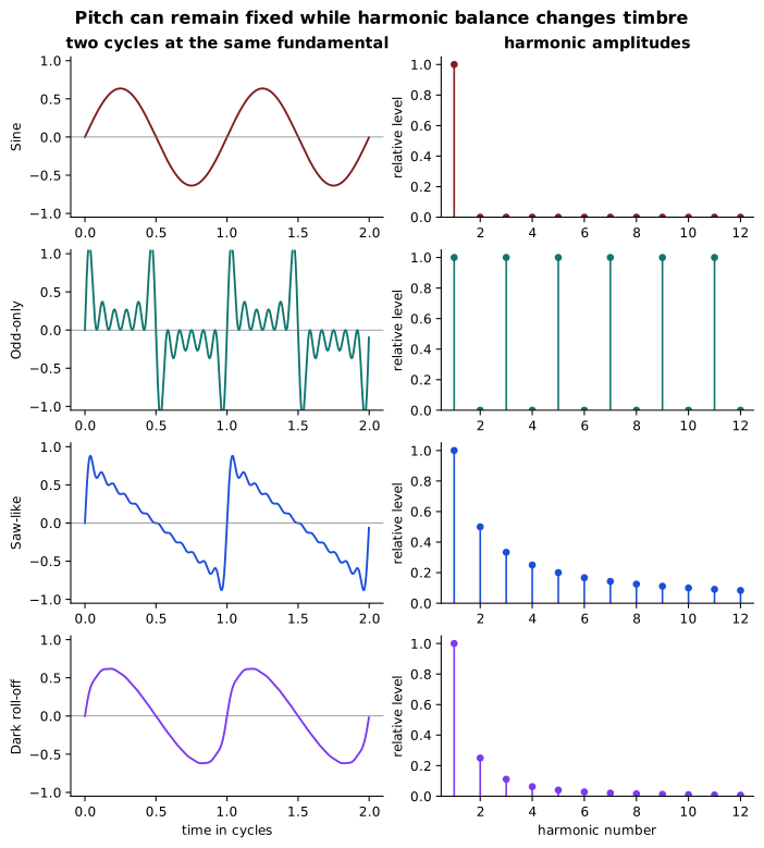
Long description. Four rows compare a waveform on
the left with harmonic amplitudes on the right. The sine row has only
harmonic 1. The odd-only row contains odd harmonics. The saw-like row
contains every harmonic with amplitude decreasing as
.
The dark row contains every harmonic with the faster decrease
.
All waveforms repeat at the same fundamental rate, but their shapes and
brightness differ. Author-generated by
assets/figures/src/ch01_harmonics.py. All four examples use
the same fundamental period and deterministic harmonic recipes.
One fixed spectrum does not describe the whole sound
A static spectrum is a frequency display captured at one moment or held fixed over time. Changing changes the colour of the sustained part of a tone. Timbre means the qualities that let us distinguish sounds beyond pitch and loudness. A fuller description also includes (Wolfe n.d.; McAdams 2019):
- the attack, or how a sound begins, and the release, or how it ends;
- how partial amplitudes change over time;
- noise and inharmonic components;
- phase relations when they affect waveform shape or brief changes called transients;
- register, or pitch range; loudness; articulation, or how notes begin, connect, and end; and musical context.
The historical apparatus gives us the harmonic idea. It does not finish the theory of timbre. Later chapters will add time, modulation, noise, performance, and perception.
The Telharmonium: make tone electrical, then distribute it
Helmholtz and Koenig treated synthesis primarily as a scientific demonstration in a room. Thaddeus Cahill pursued a much larger engineering question:
Can musical tone be generated electrically, controlled from a keyboard, and distributed from one central plant to remote listeners?
Cahill’s U.S. Patent 580,035, granted on 6 April 1897, describes an electromechanical system for producing and combining periodic electrical currents, controlling expression, and sending the result over line circuits to remote translating instruments (Cahill 1897b).

Image credit and licence. Unknown photographer, originally published in The World’s Work, June 1906. Public domain (Unknown photographer 1906).
Long description. Two operators sit at a large organ-like console with several manuals, ranks of controls, and electrical equipment behind them. The familiar keyboard interface conceals an industrial generator system elsewhere in the plant. The photograph emphasizes a recurring synthesizer pattern: a human-scale control surface may command machinery much larger or more complex than the interface suggests.
The patented sources were rotating rheotomes. A rheotome repeatedly opened and closed an electrical circuit as conducting and insulating sections rotated. Related generators ran at frequencies in harmonic ratios. Keys combined the component currents. Components called inductors resisted sudden changes in current and smoothed the harsh interruptions before the signal entered the telephone line (Cahill 1897b; Smith 2011).

Image credit and licence. Thaddeus Cahill, patent drawing, 1897. Public domain (Cahill 1897a, 1897b).
Long description. A vertically oriented patent sheet contains numbered mechanical shafts, electromagnetic structures, circuit paths, and callouts. It records an engineered system rather than a modern block diagram. The simplified diagram below extracts only the causal stages needed for this chapter.

Long description. A left-to-right flow begins with keyboard and stops, proceeds through rotating rheotomes, electrical combining and level control, telephone-line distribution, a remote receiver or horn, and finally audible tone.
Was the Telharmonium an additive synthesizer?
A careful answer has two parts.
In a broad historical sense, yes. Cahill described building complex electrical vibrations from simpler ones and arranged generators in harmonic relationships (Cahill 1897b).
By the modern sine-wave definition, not exactly. A rheotome produced an interrupted current, not an independent ideal sine wave. Cahill used inductors to smooth currents he described as abrupt and harsh. The system combined electrically generated components, but it did not give independent control over every sine wave’s amplitude, frequency, phase, and change over time as Equation 1.5 does. Smith therefore calls it only “a kind of” additive synthesis and compares it to electromechanical organs (Smith 2011).
Use the mechanism, not the label, when comparing historical and modern synthesis.
First-principles lessons for wavetable synthesis
This chapter established four foundations:
- A periodic tone can be represented as a repeatable cycle.
- A complicated cycle can be analyzed or constructed through components.
- Component balance and control are central to timbre.
- Tone generation, performer control, and distribution are separate engineering layers.
Later, a wavetable will store one period as a sequence of digital sample values instead of maintaining one physical oscillator per harmonic. The same harmonic model can describe the frequencies and amplitudes represented in that stored cycle.
Section II · Practice
Use the modelCalculate, listen, build, diagnose, and check your understanding.Mathematical concepts 1: cycles, harmonics, and finite sums
Cycle landmarks and radians
Draw one cycle. Mark its start, quarter, half, three-quarter, and end points. A radian is a unit for measuring angle. One complete cycle is radians (Puckette 2007):
| Cycle position | Angle | |
|---|---|---|
| start | ||
| one quarter | ||
| one half | ||
| three quarters | ||
| one complete cycle |
For , the quantity tells us the current angle. Frequency says how many complete journeys occur each second; phase says where the first journey begins.
Unit reasoning
A hertz is one cycle per second. Keep units visible:
Use and . Convert before taking a reciprocal.
Turn a list of amplitudes into sound
A coefficient is a number that multiplies a term in an equation. Here, each coefficient sets the amplitude of the harmonic at the same position in a list. For
list position 1 controls harmonic 1, position 2 controls harmonic 2, and position 3 controls harmonic 3. With zero phases,
The zero coefficient removes the line at ; it does not shift later list positions. A one-sided magnitude spectrum plots only zero and positive frequencies and shows the size of each component without its phase. This one has lines at and with relative heights 1.0 and 0.5.
When the waveform repeats faster than the declared fundamental
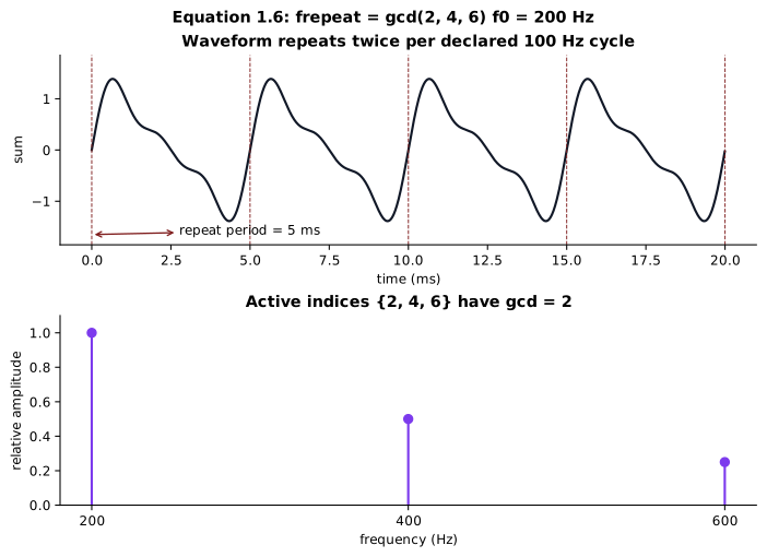
Let be the set of active harmonic numbers. The greatest common divisor (GCD) is the largest whole number that divides every number in the set. Write that number as . The selected sum’s lowest repetition frequency is

Long description. The upper panel shows the summed waveform with vertical markers every 5 ms. The lower spectrum has lines at 200, 400, and 600 Hz with amplitudes 1, 0.5, and 0.25. The active indices have greatest common divisor 2, so the lowest repetition frequency is 200 Hz.
If harmonics 2, 4, and 6 are active, then : the waveform repeats at , even if the recipe was indexed relative to a declared . If harmonic 1 is active, the greatest common divisor is necessarily 1.
Concept check: calculate and predict
Show units and intermediate steps.
- A cycle lasts 5 ms. Find its frequency in hertz.
- Evaluate at and .
- List the first five harmonics of Hz.
- Convert into a zero-phase equation and a two-line spectrum description.
- Compare recipes and . Which harmonic lines differ, and which do you predict will sound brighter after level matching?
- A recipe relative to Hz contains only harmonics 2, 4, and 6. Find its lowest repetition frequency and period.
- The sample rate is the number of digital samples processed each second. At a 48 kHz sample rate, the Nyquist frequency is half that rate, or 24 kHz. What is the largest harmonic number of a 440 Hz fundamental that remains strictly below 24 kHz (Smith 2011; Puckette 2007)?
- For each plot from Equations 1.1 through 1.7, name the axes or panels, the fixed parameters, and one prediction visible before calculation.
Worked example: design a three-harmonic tone
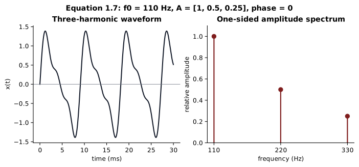
Design a tone with fundamental Hz, amplitudes
and zero starting phase.
The component frequencies are:
The signal is:

Long description. The left panel shows about three cycles of the summed waveform. The right panel has spectrum lines at 110, 220, and 330 Hz with relative amplitudes 1, 0.5, and 0.25.
Its fundamental period is:
The spectrum contains lines at 110, 220, and 330 Hz with relative heights 1.0, 0.5, and 0.25. A magnitude-only spectrum does not state the phases, although this example declares all phases zero.
Listening station 1: one pitch, four harmonic recipes
Open the Chapter 1 listening file:
assets/audio/ch01/ch01-same-pitch-different-timbres.wavThe four two-second tones are separated by silence and appear in this order:
- sine;
- equal-amplitude odd harmonics;
- saw-like harmonic roll-off;
- darker roll-off.
All use Hz. Each tone was scaled to the same root-mean-square (RMS) level, a measure of average signal strength, before short fades were applied. This scaling is called normalization (Smith 2011).
Procedure
- Keep the playback level fixed.
- For each tone, write three words describing the steady-state colour.
- Rank them from least to most bright.
- State whether the perceived pitch changes.
- Inspect the same-pitch spectrum figure and connect your brightness ranking to high-harmonic energy.
- Repeat at a lower level. Note which distinctions remain obvious.
Expected observation, not a required preference
More high-harmonic energy often supports a brighter or buzzier description, but the words are not physical units and listener descriptions can differ. What stays fixed is the fundamental frequency; only the harmonic recipe changes.
Song study 1: one melody, two spectra
LAB 01
Make the harmonic sum audible
Move one coefficient, predict the waveform and spectrum, then listen.
The current recipe contains H1 at 220 Hz with amplitude 1.00, H2 at 440 Hz with amplitude 0.50, and H3 at 660 Hz with amplitude 0.25.
Try these checks
- Set harmonic 5 to 0.50. Name the only spectrum line that must change.
- Choose Sine, then Odd only. Keep the fundamental fixed and compare pitch with colour.
- Play the melody with two recipes. Identify what remains invariant.
- Raise the fundamental. Watch every harmonic frequency rise by the same integer rule.
Read the exact source running this lab
This TypeScript calculates the sound and plots above. The coefficient list is both the equation and the spectrum.
export const SAMPLE_RATE = 48_000;
const TAU = 2 * Math.PI;

export function harmonicFrequency(fundamentalHz: number, harmonic: number) {
  return fundamentalHz * harmonic;
}

function energy(amplitudes: number[]) {
  return Math.sqrt(amplitudes.reduce((sum, amplitude) => sum + amplitude ** 2, 0)) || 1;
}

export function waveform(amplitudes: number[], points = 480) {
  const level = energy(amplitudes);
  return Array.from({ length: points }, (_, index) => {
    const cycles = 2 * index / (points - 1);
    return amplitudes.reduce(
      (sample, amplitude, harmonic) => sample + amplitude * Math.sin(TAU * (harmonic + 1) * cycles),
      0
    ) / level;
  });
}

export function renderAdditiveTone(
  fundamentalHz: number,
  amplitudes: number[],
  seconds = 1.4
) {
  const frameCount = Math.round(seconds * SAMPLE_RATE);
  const output = new Float32Array(frameCount);
  const phases = new Float64Array(amplitudes.length);
  const level = energy(amplitudes);
  const fadeFrames = Math.round(0.012 * SAMPLE_RATE);

  for (let frame = 0; frame < frameCount; frame++) {
    let sample = 0;
    for (let index = 0; index < amplitudes.length; index++) {
      const frequencyHz = harmonicFrequency(fundamentalHz, index + 1);
      if (frequencyHz >= SAMPLE_RATE / 2) continue;
      sample += amplitudes[index] * Math.sin(phases[index]);
      phases[index] = (phases[index] + TAU * frequencyHz / SAMPLE_RATE) % TAU;
    }
    const envelope = Math.min(1, frame / fadeFrames, (frameCount - 1 - frame) / fadeFrames);
    output[frame] = 0.2 * envelope * sample / level;
  }
  return output;
}

export function renderMelody(amplitudes: number[]) {
  const melody = [60, 60, 67, 67, 69, 69, 67, 65, 65, 64, 64, 62, 62, 60];
  const beats =  [ 1,  1,  1,  1,  1,  1,  2,  1,  1,  1,  1,  1,  1,  2];
  const framesPerBeat = SAMPLE_RATE * 60 / 108;
  const frameCounts = beats.map((beat) => Math.round(beat * framesPerBeat));
  const output = new Float32Array(frameCounts.reduce((sum, frames) => sum + frames, 0));
  const phases = new Float64Array(amplitudes.length);
  const level = energy(amplitudes);
  const fadeFrames = Math.round(0.005 * SAMPLE_RATE);
  let write = 0;

  melody.forEach((midi, noteIndex) => {
    const frames = frameCounts[noteIndex];
    const active = Math.floor(frames * 0.92);
    const fundamentalHz = 440 * 2 ** ((midi - 69) / 12);
    for (let frame = 0; frame < frames; frame++, write++) {
      let sample = 0;
      for (let index = 0; index < amplitudes.length; index++) {
        const frequencyHz = harmonicFrequency(fundamentalHz, index + 1);
        if (frequencyHz >= SAMPLE_RATE / 2) continue;
        sample += amplitudes[index] * Math.sin(phases[index]);
        phases[index] = (phases[index] + TAU * frequencyHz / SAMPLE_RATE) % TAU;
      }
      const envelope = frame >= active
        ? 0
        : Math.min(1, frame / fadeFrames, (active - frame) / fadeFrames);
      output[write] = 0.18 * envelope * sample / level;
    }
  });
  return output;
}
Open the browser-generated Chapter 1 melody study. It contains:
- the opening of the traditional French melody Ah! vous dirai-je, maman as a sine;
- the same notes, rhythm, tempo, and articulation, meaning how each note begins, connects, and ends, with amplitudes ;
- an original eight-note A/B ostinato, or repeating musical pattern, on A3 that alternates two harmonic recipes.
The melody begins C4 C4 G4 G4 A4 A4 G4 and continues
F4 F4 E4 E4 D4 D4 C4. It predates Mozart; his public-domain
variations provide a historical score reference, but this book does not
credit him as composer of the tune (Mozart 1778). The audio is newly synthesized and
monophonic, meaning it plays one note at a time. It is
not a borrowed recording or modern arrangement. The two recipes are
scaled from their coefficients so that their sustained RMS levels are
comparable. Each note has a short fade-in and fade-out, which can still
cause small measured differences.
Listening questions
- Which shared features, such as notes, rhythm, tempo, or articulation, make the two passes recognizably the same melody?
- Which pass makes repeated notes easier to separate, and is that caused by spectrum or articulation?
- Does the four-harmonic recipe change melodic contour, pitch center, or only tone colour?
- In the final ostinato, can alternating timbre alone create a call and response?
- Hum the melody after stopping playback. Which properties survive without the synthesizer timbre?
Figure lab 1: reproduce the plots
Run:
python3 assets/figures/src/ch01_harmonics.pyVerify that it regenerates:
assets/figures/svg/ch01-harmonic-construction.svg
assets/figures/svg/ch01-same-pitch-different-timbres.svg
assets/audio/ch01/ch01-same-pitch-different-timbres.wav
Then change only the amplitude of harmonic 5 in one recipe. Before listening, predict how the time waveform and spectrum must change. Regenerate, listen, and record whether the perceptual change was as large as expected.
Browser lab 1: make the mathematics audible
Use the interactive additive-synthesis lab on this page. Change one coefficient, listen at a safe level, and compare the plotted waveform with the harmonic recipe. The TypeScript displayed in the lab is byte-identical to the source the browser executes.
- verify
period_seconds(250.0)andharmonic_frequency(110.0, 5)by hand; - change one amplitude coefficient and predict the spectrum before listening;
- add a sixth harmonic, then state the fundamental frequency at which it would reach or exceed the Nyquist frequency as pitch rises;
- transpose the melody while preserving its rhythm and coefficient pattern.
Practice: complete a harmonic recipe
A tone has fundamental Hz and the partially specified recipe:
harmonic:   1      2      3      4
frequency:  ?      ?      ?      ?
amplitude:  1.0    0.4    0.2    0.1
phase: 0 0 0 0- Complete the frequencies without returning to Equation 1.4.
- Write the four-term signal, leaving the common factor visible.
- Sketch its one-sided amplitude spectrum.
- Predict how removing harmonic 2 changes the spectrum before listening.
Musical application 1: harmonic call and response
Use the Chapter 1 Python script, an additive synthesizer, or any instrument that lets you control harmonic balance.
- Make Tone A from harmonics 1, 2, and 3.
- Make Tone B from harmonics 1, 3, and 5.
- Match their fundamental, duration, and approximate RMS level, which measures average signal strength.
- Perform or render an eight-event phrase alternating A and B while keeping pitch fixed.
- Repeat with the same rhythm but let pitch move while timbre remains fixed.
- Write which dimension (pitch, rhythm, or harmonic colour) carried the call-and-response identity in each version.
The goal is not to find one spectrum that is always best. It is to hear how changing timbre alone can organize a phrase.
Challenge: diagnose the explanation
A student writes:
“The first overtone is the first harmonic. Every partial is harmonic. The Telharmonium generated six perfect sine waves and therefore worked exactly like modern additive synthesis.”
Mark each incorrect clause. For every correction, identify whether the mistake is vocabulary, historical evidence, or DSP modeling.
Chapter 1 readiness gate
Commit answers before consulting the answer invariants.
- For , identify amplitude, frequency, phase, period, and angular frequency.
- A periodic tone has Hz. List its first six harmonics and identify the first overtone.
- Write a finite three-harmonic signal with amplitudes 1, 0.5, and 0.25 and zero phases.
- What does each line in a one-sided amplitude spectrum encode, and what does a magnitude-only plot omit?
- Explain the Koenig-built Helmholtz apparatus as a signal-flow system.
- Is the Telharmonium modern additive synthesis? Give the two-part answer supported by historical evidence.
Chapter 1 invariants
- Frequency is the reciprocal of period.
- Harmonic lies at .
- The fundamental is harmonic 1; the first overtone is normally harmonic 2.
- A finite additive model sums controlled sinusoidal components.
- A magnitude spectrum omits phase and temporal development.
- Harmonic balance strongly affects steady-state timbre but does not exhaust timbre.
- Historical terminology must be qualified against the actual mechanism.
Chapter 1 glossary
| Term | Working definition |
|---|---|
| Additive synthesis | Building one sound by adding controlled components (Smith 2011; Puckette 2007). |
| Aliasing | A false lower frequency produced when a sampled signal contains a frequency at or above the Nyquist limit (Smith 2011; Puckette 2007). |
| Amplitude | A measure or coefficient of signal size. For the sine waves in this chapter, it is the peak distance from zero (Puckette 2007). |
| Angular frequency | Phase advance per second in radians; . |
| Coefficient | A number that multiplies a term. In a harmonic recipe, each coefficient sets one harmonic’s amplitude. |
| Cycle | One complete repetition of a periodic waveform. |
| Frequency | Cycles per second, measured in hertz. |
| Fundamental | Lowest declared harmonic reference; harmonic 1. |
| Harmonic | A component at an integer multiple of . |
| Magnitude spectrum | A display of component frequencies and their sizes without phase or change over time. A one-sided spectrum shows only zero and positive frequencies (Smith 2011). |
| Nyquist frequency | Half the sample rate; sampled components must remain below it to avoid direct aliasing. |
| Overtone | A component above the fundamental; the first overtone is normally harmonic 2. |
| Partial | Any component of a tone, whether harmonic or inharmonic. |
| Normalization | Scaling signals to a chosen level so they can be compared more fairly. |
| Period | Time for one repetition; . |
| Phase | Position within a cycle, measured as an angle. |
| Radian | A unit for measuring angle. One complete cycle is radians (Puckette 2007). |
| Rheotome | Cahill’s rotating electrical source, which repeatedly opened and closed a circuit (Cahill 1897b). |
| Root-mean-square (RMS) level | A measure of a signal’s average strength over time (Smith 2011). |
| Sample rate | The number of digital samples stored or processed each second (Puckette 2007). |
| Sinusoid | The mathematical term for a sine wave: a repeating waveform described by amplitude, frequency, and phase (Smith 2011; Puckette 2007). |
| Timbre | The qualities that let us distinguish sounds beyond pitch and loudness, including spectrum and change over time (McAdams 2019; Wolfe n.d.). |
IMPLEMENTATION NOTEBOOK
Chapter 1 source and generated output
Each website-owned Python or Mermaid source appears beside the deterministic output it generated. The browser lab above publishes its executed TypeScript separately.
SOURCE AND OUTPUT
Harmonic figures and listening study
This Python program generates both harmonic figures and the four-part level-matched listening file.
Output
Source
ch01_harmonics.py
assets/figures/src/ch01_harmonics.pyPython
#!/usr/bin/env python3
"""Generate Chapter 1 harmonic figures and the level-matched listening file."""

from __future__ import annotations

import wave
from pathlib import Path

import matplotlib
matplotlib.use("Agg")
import matplotlib.pyplot as plt
import numpy as np

ROOT = Path(__file__).resolve().parents[3]
SVG = ROOT / "assets/figures/svg"
AUDIO = ROOT / "assets/audio/ch01"
SVG.mkdir(parents=True, exist_ok=True)
AUDIO.mkdir(parents=True, exist_ok=True)

plt.rcParams.update(
    {
        "font.family": "DejaVu Sans",
        "font.size": 9,
        "axes.spines.top": False,
        "axes.spines.right": False,
        "axes.titleweight": "bold",
        "svg.fonttype": "none",
    }
)
COLORS = ["#7F1D1D", "#0F766E", "#1D4ED8", "#7C3AED", "#B45309"]


def harmonic_sum(phase: np.ndarray, amplitudes: list[float], phases: list[float] | None = None) -> np.ndarray:
    phases = phases or [0.0] * len(amplitudes)
    result = np.zeros_like(phase, dtype=float)
    for index, (amplitude, offset) in enumerate(zip(amplitudes, phases), start=1):
        result += amplitude * np.sin(2 * np.pi * index * phase + offset)
    return result


def normalize_rms(signal: np.ndarray, target: float = 0.18) -> np.ndarray:
    signal = signal - np.mean(signal)
    rms = np.sqrt(np.mean(signal**2))
    return signal * (target / rms) if rms else signal


def fade(signal: np.ndarray, sample_rate: int, seconds: float = 0.03) -> np.ndarray:
    frames = min(int(sample_rate * seconds), len(signal) // 2)
    ramp = np.linspace(0.0, 1.0, frames)
    signal = signal.copy()
    signal[:frames] *= ramp
    signal[-frames:] *= ramp[::-1]
    return signal


def write_wav(path: Path, signal: np.ndarray, sample_rate: int = 48_000) -> None:
    signal = np.clip(signal, -0.98, 0.98)
    pcm = np.round(signal * 32767).astype("<i2")
    with wave.open(str(path), "wb") as output:
        output.setnchannels(1)
        output.setsampwidth(2)
        output.setframerate(sample_rate)
        output.writeframes(pcm.tobytes())


# Figure 1: progressively combine a harmonic series.
phase = np.linspace(0.0, 2.0, 1600, endpoint=False)
amplitudes = [1.0, 0.50, 0.33, 0.25, 0.20]
fig, axes = plt.subplots(3, 1, figsize=(7.2, 6.5), sharex=True, constrained_layout=True)
for count, axis in zip([1, 3, 5], axes):
    partials = [amplitudes[k - 1] * np.sin(2 * np.pi * k * phase) for k in range(1, count + 1)]
    for k, partial in enumerate(partials, start=1):
        axis.plot(phase, partial, color=COLORS[(k - 1) % len(COLORS)], alpha=0.28, linewidth=0.8)
    total = np.sum(partials, axis=0)
    axis.plot(phase, total, color="#111827", linewidth=1.8, label="sum")
    axis.axhline(0, color="#6B7280", linewidth=0.5)
    axis.set_ylabel("amplitude")
    axis.set_title(f"Fundamental plus {count - 1} overtone{'s' if count != 2 else ''}")
axes[-1].set_xlabel("time in cycles of the fundamental")
fig.suptitle("A complex periodic tone built from harmonically related sinusoids", fontsize=12, fontweight="bold")
fig.savefig(SVG / "ch01-harmonic-construction.svg", bbox_inches="tight")
plt.close(fig)

# Figure 2: same pitch, different harmonic recipes.
recipes = {
    "Sine": [1.0] + [0.0] * 11,
    "Odd-only": [1.0 if k % 2 else 0.0 for k in range(1, 13)],
    "Saw-like": [1.0 / k for k in range(1, 13)],
    "Dark roll-off": [1.0 / (k * k) for k in range(1, 13)],
}
fig, axes = plt.subplots(len(recipes), 2, figsize=(7.2, 8.0), constrained_layout=True)
short_phase = np.linspace(0.0, 2.0, 1200, endpoint=False)
for row, (name, recipe) in enumerate(recipes.items()):
    waveform = normalize_rms(harmonic_sum(short_phase, recipe), 0.45)
    axes[row, 0].plot(short_phase, waveform, color=COLORS[row], linewidth=1.4)
    axes[row, 0].axhline(0, color="#6B7280", linewidth=0.5)
    axes[row, 0].set_ylabel(name)
    axes[row, 0].set_ylim(-1.05, 1.05)
    harmonics = np.arange(1, len(recipe) + 1)
    markerline, stemlines, baseline = axes[row, 1].stem(harmonics, recipe, basefmt=" ")
    plt.setp(markerline, color=COLORS[row], markersize=4)
    plt.setp(stemlines, color=COLORS[row], linewidth=1.2)
    axes[row, 1].set_xlim(0.5, 12.5)
    axes[row, 1].set_ylim(0.0, 1.05)
    axes[row, 1].set_ylabel("relative level")
axes[0, 0].set_title("two cycles at the same fundamental")
axes[0, 1].set_title("harmonic amplitudes")
axes[-1, 0].set_xlabel("time in cycles")
axes[-1, 1].set_xlabel("harmonic number")
fig.suptitle("Pitch can remain fixed while harmonic balance changes timbre", fontsize=12, fontweight="bold")
fig.savefig(SVG / "ch01-same-pitch-different-timbres.svg", bbox_inches="tight")
plt.close(fig)

# Listening file: four two-second, level-matched tones separated by silence.
sample_rate = 48_000
segment_seconds = 2.0
silence = np.zeros(int(sample_rate * 0.45))
t = np.arange(int(sample_rate * segment_seconds)) / sample_rate
fundamental = 220.0
segments = []
for recipe in recipes.values():
    signal = np.zeros_like(t)
    for harmonic, amplitude in enumerate(recipe, start=1):
        signal += amplitude * np.sin(2 * np.pi * harmonic * fundamental * t)
    signal = fade(normalize_rms(signal), sample_rate)
    segments.extend([signal, silence])
write_wav(AUDIO / "ch01-same-pitch-different-timbres.wav", np.concatenate(segments[:-1]), sample_rate)

print("Generated Chapter 1 figures and audio.")
SOURCE AND OUTPUT
Equation figures
One deterministic Python program renders the exact plots paired with the numbered formulas.
Output
Source
formula_visuals_ch01.py
assets/figures/src/formula_visuals_ch01.pyPython
#!/usr/bin/env python3
"""Generate deterministic visuals for the numbered formulas in Chapter 1."""

from __future__ import annotations

from pathlib import Path

import matplotlib

matplotlib.use("Agg")
import matplotlib.pyplot as plt
import numpy as np

ROOT = Path(__file__).resolve().parents[3]
SVG = ROOT / "assets/figures/svg"
SVG.mkdir(parents=True, exist_ok=True)

RED = "#7F1D1D"
TEAL = "#0F766E"
BLUE = "#1D4ED8"
PURPLE = "#7C3AED"
GOLD = "#B45309"
GRAY = "#6B7280"
BLACK = "#111827"

plt.rcParams.update(
    {
        "font.family": "DejaVu Sans",
        "font.size": 9,
        "axes.spines.top": False,
        "axes.spines.right": False,
        "axes.titleweight": "bold",
        "svg.fonttype": "none",
    }
)


def save(fig: plt.Figure, filename: str) -> None:
    fig.savefig(SVG / filename, bbox_inches="tight")
    plt.close(fig)


def zero_line(axis: plt.Axes) -> None:
    axis.axhline(0.0, color=GRAY, linewidth=0.6)


# Equation 1.1: amplitude, frequency, period, and phase in one sinusoid.
t = np.linspace(0.0, 1.25, 1600)
amplitude = 0.8
frequency = 2.0
phase = np.pi / 4
signal = amplitude * np.sin(2 * np.pi * frequency * t + phase)
unshifted = amplitude * np.sin(2 * np.pi * frequency * t)
fig, axis = plt.subplots(figsize=(7.2, 3.2), constrained_layout=True)
axis.plot(t, signal, color=RED, linewidth=2.0, label="φ = π/4")
axis.plot(t, unshifted, color=GRAY, linewidth=1.0, linestyle="--", label="φ = 0 reference")
axis.axhline(amplitude, color=TEAL, linewidth=0.8, linestyle=":", label="±A = ±0.8")
axis.axhline(-amplitude, color=TEAL, linewidth=0.8, linestyle=":")
axis.annotate("T = 1/f = 0.5 s", xy=(0.25, -1.02), xytext=(0.75, -1.02), ha="center", va="center", arrowprops={"arrowstyle": "<->", "color": BLACK})
axis.set(xlabel="time t (s)", ylabel="s(t)", xlim=(0, 1.25), ylim=(-1.15, 1.15), title="Equation 1.1: A = 0.8, f = 2 Hz, φ = π/4")
axis.legend(frameon=False, ncol=3, loc="upper right")
save(fig, "eq-1-1-sinusoid.svg")

# Equation 1.2: angular phase advances linearly and the sine reads that angle.
omega = 4 * np.pi
angle = omega * t + phase
fig, axes = plt.subplots(2, 1, figsize=(7.2, 4.8), sharex=True, constrained_layout=True)
axes[0].plot(t, angle / (2 * np.pi), color=BLUE, linewidth=2)
axes[0].set(ylabel="phase θ / 2π (cycles)", title="Angle advances at ω = 4π rad/s")
axes[1].plot(t, amplitude * np.sin(angle), color=RED, linewidth=1.8)
zero_line(axes[1])
axes[1].set(xlabel="time t (s)", ylabel="s(t)", title="The sine converts angle into amplitude")
fig.suptitle("Equation 1.2: s(t) = A sin(ωt + φ), A = 0.8, ω = 4π, φ = π/4", fontweight="bold")
save(fig, "eq-1-2-angular-frequency.svg")

# Equation 1.3: frequency is the reciprocal of period.
period_ms = np.linspace(1.0, 20.0, 800)
frequency_hz = 1000.0 / period_ms
fig, axis = plt.subplots(figsize=(7.2, 3.2), constrained_layout=True)
axis.plot(period_ms, frequency_hz, color=BLUE, linewidth=2)
for x, y, label in [(10.0, 100.0, "10 ms ↔ 100 Hz"), (1000 / 440, 440.0, "2.27 ms ↔ 440 Hz")]:
    axis.scatter([x], [y], color=RED, zorder=3)
    axis.annotate(label, (x, y), xytext=(8, 8), textcoords="offset points")
axis.set(xlabel="period T (ms)", ylabel="frequency f (Hz)", xlim=(1, 20), ylim=(0, 1020), title="Equation 1.3: shorter periods produce higher frequencies")
save(fig, "eq-1-3-period-frequency.svg")

# Equation 1.4: harmonic frequency grows linearly with harmonic number.
fundamental = 110.0
harmonic = np.arange(1, 7)
harmonic_hz = harmonic * fundamental
fig, axis = plt.subplots(figsize=(7.2, 3.2), constrained_layout=True)
markerline, stemlines, _ = axis.stem(harmonic, harmonic_hz, basefmt=" ")
plt.setp(markerline, color=RED, markersize=6)
plt.setp(stemlines, color=RED, linewidth=1.6)
for k, value in zip(harmonic, harmonic_hz):
    axis.annotate(f"{value:.0f}", (k, value), xytext=(0, 7), textcoords="offset points", ha="center")
axis.set(xticks=harmonic, xlabel="harmonic number k", ylabel="frequency fk (Hz)", ylim=(0, 720), title="Equation 1.4: fk = k f0 with f0 = 110 Hz")
save(fig, "eq-1-4-harmonic-family.svg")

# Equation 1.6: active harmonic indices 2, 4, and 6 repeat at 2f0.
fundamental = 100.0
active = np.array([2, 4, 6])
amplitudes = np.array([1.0, 0.5, 0.25])
t_short = np.linspace(0.0, 0.020, 2400, endpoint=False)
components = amplitudes[:, None] * np.sin(2 * np.pi * active[:, None] * fundamental * t_short)
summed = components.sum(axis=0)
fig, axes = plt.subplots(2, 1, figsize=(7.2, 5.2), constrained_layout=True)
axes[0].plot(t_short * 1000, summed, color=BLACK, linewidth=1.6)
for boundary in np.arange(0, 20.1, 5):
    axes[0].axvline(boundary, color=RED, linewidth=0.7, linestyle="--")
axes[0].annotate("repeat period = 5 ms", xy=(0, -1.65), xytext=(5, -1.65), ha="center", arrowprops={"arrowstyle": "<->", "color": RED})
axes[0].set(xlabel="time (ms)", ylabel="sum", ylim=(-1.85, 1.85), title="Waveform repeats twice per declared 100 Hz cycle")
markerline, stemlines, _ = axes[1].stem(active * fundamental, amplitudes, basefmt=" ")
plt.setp(markerline, color=PURPLE, markersize=6)
plt.setp(stemlines, color=PURPLE, linewidth=1.6)
axes[1].set(xlabel="frequency (Hz)", ylabel="relative amplitude", xticks=active * fundamental, ylim=(0, 1.1), title="Active indices {2, 4, 6} have gcd = 2")
fig.suptitle("Equation 1.6: frepeat = gcd(2, 4, 6) f0 = 200 Hz", fontweight="bold")
save(fig, "eq-1-6-gcd-repetition.svg")

# Equation 1.7: exact worked three-harmonic signal and spectrum.
fundamental = 110.0
amplitudes = np.array([1.0, 0.5, 0.25])
t_short = np.linspace(0.0, 0.030, 2400, endpoint=False)
components = amplitudes[:, None] * np.sin(2 * np.pi * np.arange(1, 4)[:, None] * fundamental * t_short)
summed = components.sum(axis=0)
fig, axes = plt.subplots(1, 2, figsize=(7.2, 3.3), constrained_layout=True)
axes[0].plot(t_short * 1000, summed, color=BLACK, linewidth=1.5)
zero_line(axes[0])
axes[0].set(xlabel="time (ms)", ylabel="x(t)", title="Three-harmonic waveform")
markerline, stemlines, _ = axes[1].stem([110, 220, 330], amplitudes, basefmt=" ")
plt.setp(markerline, color=RED, markersize=6)
plt.setp(stemlines, color=RED, linewidth=1.6)
axes[1].set(xlabel="frequency (Hz)", ylabel="relative amplitude", xticks=[110, 220, 330], ylim=(0, 1.1), title="One-sided amplitude spectrum")
fig.suptitle("Equation 1.7: f0 = 110 Hz, A = [1, 0.5, 0.25], phase = 0", fontweight="bold")
save(fig, "eq-1-7-worked-tone.svg")

print("Generated Chapter 1 formula visuals.")
SOURCE AND OUTPUT
Signal diagrams
The Mermaid sources produce the harmonic-synthesis and Telharmonium signal diagrams.
Output

Source
ch01-harmonic-synthesis.mmd
assets/diagrams/src/ch01-harmonic-synthesis.mmdMermaid
flowchart LR
    F1[Fundamental<br/>f₀] --> G1[Level<br/>A₁]
    F2[Second<br/>harmonic<br/>2f₀] --> G2[Level<br/>A₂]
    F3[Third<br/>harmonic<br/>3f₀] --> G3[Level<br/>A₃]
    FN[Higher<br/>harmonics<br/>kf₀] --> GN[Level<br/>Ak]
    G1 --> SUM((Sum))
    G2 --> SUM
    G3 --> SUM
    GN --> SUM
    SUM --> TONE[Periodic<br/>tone<br/>distinctive<br/>timbre]
ch01-telharmonium-flow.mmd
assets/diagrams/src/ch01-telharmonium-flow.mmdMermaid
flowchart LR
    K[Keyboard<br/>stops] --> R[Rheotomes<br/>periodic<br/>signals]
    R --> C[Combine<br/>level]
    C --> L[Telephone-line<br/>distribution]
    L --> H[Remote<br/>horn]
    H --> A[Audible<br/>tone]
Chapter 1 Answers and Fault Invariants
Chapter 1 mathematical-practice answers
- , so Hz.
- The values are respectively.
- 82.5, 165, 247.5, 330, and 412.5 Hz.
- ; spectrum lines occur at with height 1 and with height 0.5.
- The first recipe contains harmonics 1–4; the second contains only 1 and 3. After level matching, the first will usually be predicted brighter because it retains harmonics 2 and 4. Listening language may differ; the spectral difference may not.
- , so the lowest repetition is 200 Hz and its period is 5 ms.
- Require , so and the largest integer harmonic is 54.
- A valid response identifies every axis or panel, copies the stated parameter values, and links one visual feature to the formula. Examples include period shrinking as frequency rises, equal harmonic-index steps adding , and the 2/4/6 sum repeating at .
Chapter 1 readiness answers
- ; Hz; radians; s = 4 ms; rad/s.
- 110, 220, 330, 440, 550, and 660 Hz. The first overtone is 220 Hz, the second harmonic.
- One valid answer is .
- Each line gives a component frequency and magnitude under the declared normalization. A magnitude-only plot omits phase and temporal envelopes.
- Sustained tuning forks generate components; matched resonators and keyboard-operated shutters control audibility; sound pressure in the room sums the active components.
- Broadly additive: Cahill combined harmonic-related electrical components. Not equivalent to modern sinusoidal additive synthesis: rheotome currents were nonsinusoidal, required smoothing, and did not expose the general independent sinusoidal parameter set of Equation 1.5.
Chapter 1 faded and musical-station invariants
- The frequencies are 220, 440, 660, and 880 Hz.
- One valid signal is .
- Removing harmonic 2 deletes only the 440 Hz spectrum line in this model; it does not change the declared fundamental.
- Acceptable musical proof includes two level-matched same-pitch recipes, an eight-event render or performance, and a written comparison of which dimension carries phrase identity.
Chapter 1 fault invariant
- The first overtone is not the first harmonic under normal counting.
- Not every partial is harmonic.
- The patent does not describe six independently arbitrary perfect sine oscillators.
- The historical and modern meanings of additive synthesis must remain distinct.